This blog shows how you can load data from an Iceberg table into PyArrow or DuckDB using PyIceberg. The code is publicly available on the docker-spark-iceberg Github repository that contains a full docker-compose stack of Apache Spark with Iceberg support, MinIO as a storage backend, and a REST catalog as a catalog. This is a companion piece to our PyIceberg video 0.2.1 video. It requires docker and docker-compose installed.
First, let’s clone the repository and bring up the stack:
git clone https://github.com/tabular-io/docker-spark-iceberg.git
cd docker-spark-iceberg
docker-compose up
It takes a couple of seconds to download the images and start all the services. Next, open up a web browser to go to the Jupyter notebook UI that comes with the Spark images.
Use the notebook PyIceberg - Getting Started.ipynb to create the table nyc.taxis:
%%sql
CREATE DATABASE IF NOT EXISTS nyc;

CREATE TABLE IF NOT EXISTS nyc.taxis (
    VendorID              bigint,
    tpep_pickup_datetime  timestamp,
    tpep_dropoff_datetime timestamp,
    passenger_count       double,
    trip_distance         double,
    RatecodeID            double,
    store_and_fwd_flag    string,
    PULocationID          bigint,
    DOLocationID          bigint,
    payment_type          bigint,
    fare_amount           double,
    extra                 double,
    mta_tax               double,
    tip_amount            double,
    tolls_amount          double,
    improvement_surcharge double,
    total_amount          double,
    congestion_surcharge  double,
    airport_fee           double
)
USING iceberg
PARTITIONED BY (days(tpep_pickup_datetime))
It is always a good idea to think about how to partition the data. With Iceberg you can always change this later, but having a good partition column that matches with your access pattern can dramatically increase query performance. Iceberg will be able to skip files, which is also beneficial for PyIceberg since it will open fewer files, and consume less memory.
Let’s load some data:
from pyspark.sql import SparkSession
spark = SparkSession.builder.appName("Jupyter").getOrCreate()

for filename in [
    "yellow_tripdata_2022-04.parquet",
    "yellow_tripdata_2022-03.parquet",
    "yellow_tripdata_2022-02.parquet",
    "yellow_tripdata_2022-01.parquet",
    "yellow_tripdata_2021-12.parquet",
]:
    df = spark.read.parquet(f"/home/iceberg/data/{filename}")
    df.write.mode("append").saveAsTable("nyc.taxis")
Using PySpark you don’t need to use a full-blown JVM to interact with the Iceberg tables.
Load data into PyArrow
First, a catalog needs to be defined to load a table. The docker-compose comes with a REST catalog that’s used to store the metadata. Instead of programmatically providing the location and credentials, you can also set a configuration file.
from pyiceberg.catalog import load_catalog

catalog = load_catalog('default', **{
    'uri': 'http://rest:8181',
    's3.endpoint': 'http://minio:9000',
    's3.access-key-id': 'admin',
    's3.secret-access-key': 'password',
})
Now retrieve the table using the catalog:
tbl = catalog.load_table('nyc.taxis')
Using the reference of the table, create a TableScan to fetch the data:
from pyiceberg.expressions import GreaterThanOrEqual

sc = tbl.scan(row_filter=GreaterThanOrEqual("tpep_pickup_datetime", "2022-01-01T00:00:00.000000+00:00"))
The TableScan has a rich API to do filtering and column selection. Both limiting the number of rows and columns will lead to lower memory consumption, and therefore it is advised to only retrieve the data that you need:
df = sc.to_arrow().to_pandas()
Now the data is in memory, and let’s look at the dataframe using df.info():
RangeIndex: 12671129 entries, 0 to 12671128
Data columns (total 19 columns):
 #   Column                 Dtype
---  ------                 -----
 0   VendorID               int64
 1   tpep_pickup_datetime   datetime64[ns, UTC]
 2   tpep_dropoff_datetime  datetime64[ns, UTC]
 3   passenger_count        float64
 4   trip_distance          float64
 5   RatecodeID             float64
 6   store_and_fwd_flag     object
 7   PULocationID           int64
 8   DOLocationID           int64
 9   payment_type           int64
 10  fare_amount            float64
 11  extra                  float64
 12  mta_tax                float64
 13  tip_amount             float64
 14  tolls_amount           float64
 15  improvement_surcharge  float64
 16  total_amount           float64
 17  congestion_surcharge   float64
 18  airport_fee            float64
dtypes: datetime64[ns, UTC](2), float64(12), int64(4), object(1)
memory usage: 1.8+ GB
The table can be of petabyte size, but using PyIceberg the memory size will be proportional to the data that’s being loaded using the TableScan. This doesn’t mean that you shouldn’t filter any further. Let’s make a simple plot:
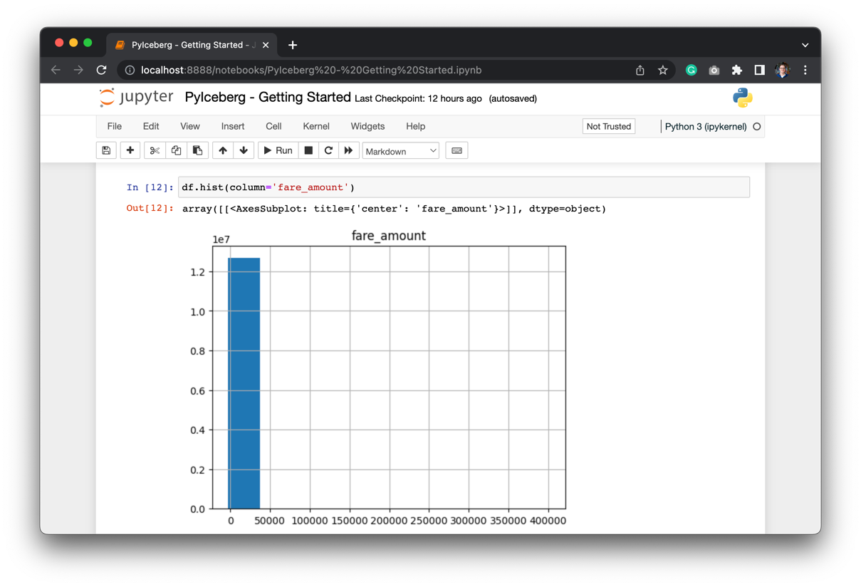
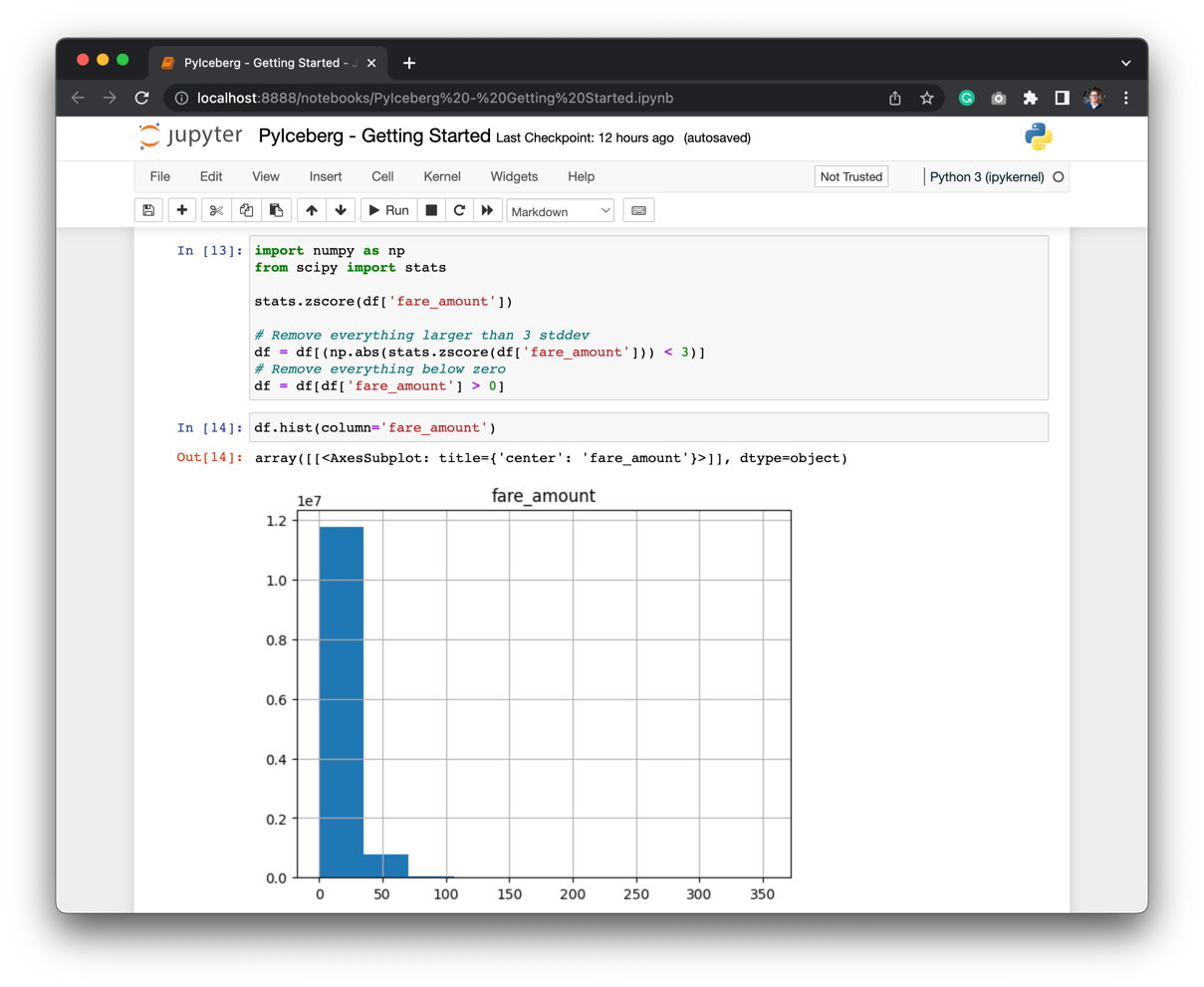
The data contains outliers. Let’s filter out the outliers:
import numpy as np
from scipy import stats

stats.zscore(df['fare_amount'])

# Remove everything larger than 3 stddev
df = df[(np.abs(stats.zscore(df['fare_amount'])) < 3)]
# Remove everything below zero
df = df[df['fare_amount'] > 0]
The result is still a long-tail distribution, but the distribution is much less skewed than before:
PyIceberg allows the users to quickly iterate of different parts of the dataset, and load the data that’s needed for the analysis.
Query using DuckDB
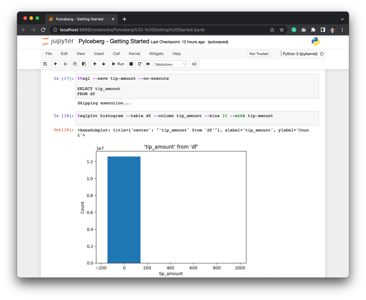
With PyArrow also comes support from DuckDB. If you’re a SQL enthousiast like me, then you’ll love DuckDB. The first cell prepares the query:
%%sql --save tip-amount --no-execute

SELECT tip_amount
FROM df
This query isn’t directly executed, but will be referenced in the next cell where the plot is defined:
%sqlplot histogram --table df --column tip_amount --bins 22 --with tip-amount
Which gives a very skewed dataset. This is likely an outlier since a 400k tip doesn’t sound reasonable for a taxi ride.
Let’s filter the data in a similar way as with Python, but now in SQL:
%%sql --save tip-amount-filtered --no-execute

WITH tip_amount_stddev AS (
    SELECT STDDEV_POP(tip_amount) AS tip_amount_stddev
    FROM df
)

SELECT tip_amount
FROM df, tip_amount_stddev
WHERE tip_amount > 0
  AND tip_amount < tip_amount_stddev * 3
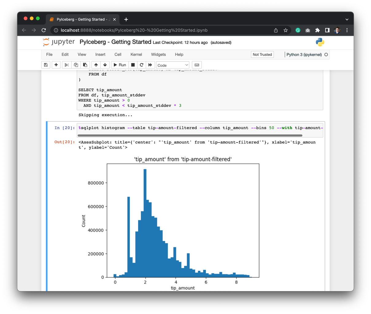
And run the plot again:
%sqlplot histogram --table tip-amount-filtered --column tip_amount --bins 50 --with tip-amount-filtered
The distribution of tips is around 2USD:
I’d recommend firing up the stack and running the queries to make the plots interactive.
Hope you’ve learned something about PyIceberg today. If you run into anything, please don’t hesitate to reach out on the #python channel on Slack, or create an issue on Github.