Polars
Polars is a lightning fast DataFrame library/in-memory query engine. Its embarrassingly parallel execution, cache efficient algorithms and expressive API makes it perfect for efficient data wrangling and data pipelines. Recently, PyIceberg has been added to ingest data from Apache Iceberg tables. Polars is a popular choice for data preprocessing, analytics and machine learning.
Polars is written in Rust, but has a Python API to make it easy to use. This allowed PyIceberg to be integrated quite easily. However, in the future it would be to replace the PyIceberg implementation with iceberg-rust for performance reasons.
Let’s get cracking!
Make sure that you install Polars with the PyIceberg extension:
pip install 'polars[pyiceberg]'
That’s all! Now you can create dataframes from PyIceberg tables directly:
import polars as pl

df = pl.scan_iceberg(
    "s3://bucket/path/to/iceberg-table/metadata.json",
    storage_options={
        "s3.region": "eu-central-1",
        "s3.access-key-id": "AKI...",
        "s3.secret-access-key": "19CO...",
    }
)
Since it is backed by PyIceberg, it offers the same features. For example, to read from GCS:
import polars as pl

df = pl.scan_iceberg(
    "gs://bucket/path/to/iceberg-table/metadata.json",
    storage_options={
        "gcs.project-id": "my-gcp-project",
        "gcs.oauth.token": "ya29.dr.AfM...",
    }
)
And Azure:
import polars as pl

df = pl.scan_iceberg(
    "az://container/path/to/iceberg-table/metadata.json",
    storage_options={
        "adlfs.account-name": "AZURE_STORAGE_ACCOUNT_NAME",
        "adlfs.account-key": "AZURE_STORAGE_ACCOUNT_KEY",
    }
)
For all the configuration options, please check the PyIceberg configuration page.
Loading a table directly from a metadata file is a quick way to get started, but with Iceberg the recommended way to access your data is through a catalog.
To give it a quick try, you can create a free account on Tabular. Create a credential through the web UI and add that to the local ~/.pyiceberg.yaml file:
default-catalog: default

catalog:
    default:
        uri: https://api.dev.tabulardata.io/ws/
        credential: t--qP....
        warehouse: examples
Now the catalog is set. You can define multiple catalogs if you want to easily switch between them.
>>> from pyiceberg.catalog import load_catalog
>>> catalog = load_catalog('default')
Let’s list the databases in the catalog:
>>> catalog.list_namespaces()
Returns:
[
    ('default',),
    ('examples',)
]
Or the tables in the database:
>>> catalog.list_tables('examples')
Returns:
[
    ('examples', 'backblaze_drive_stats'),
    ('examples', 'nyc_taxi_locations'),
    ('examples', 'nyc_taxi_yellow')
]
Let’s do a query from a table:
>>> tbl = catalog.load_table('examples.nyc_taxi_yellow')
>>> tbl
This shows a summary of the table:
nyc_taxi_yellow (
  1: vendor_id: optional int (TPEP provider code; 1=Creative Mobile Technologies, LLC; 2=VeriFone Inc.),
  2: pickup_time: optional timestamptz (Date and time when the meter was engaged),
  3: pickup_location_id: optional int (Location ID where the meter was engaged),
  4: dropoff_time: optional timestamptz (Date and time when the meter was disengaged),
  5: dropoff_location_id: optional int (Location ID where the meter was disengaged),
  6: passenger_count: optional int (Number of passengers in the vehicle (driver entered)),
  7: trip_distance: optional double (Elapsed trip distance in miles reported by the meter),
  8: ratecode_id: optional int (Final rate code in effect when the trip ended),
  9: payment_type: optional int (How the passgener paid; 1=Credit card; 2=Cash; 3=No charge; 4=Dispute; 5=Unknown; 6=Voided trip),
  10: total_amount: optional double (Total amount charged to passengers; cash tips not included),
  11: fare_amount: optional double (Time-and-distance fare in USD calculated by the meter),
  12: tip_amount: optional double (Tip amount; automatically populated for credit card tips; cash tips not included),
  13: tolls_amount: optional double (Total amount of all tolls paid in trip),
  14: mta_tax: optional double (MTA tax automatically triggered based on the metered rate in use; $0.50),
  15: improvement_surcharge: optional double (Improvement surcharge assessed trips at the flag drop; $0.30),
  16: congestion_surcharge: optional double (Congestion surcharge),
  17: airport_fee: optional double (Airport fee),
  18: extra_surcharges: optional double (Misc. extras and surcharges; $0.50 and $1.00 rush hour and overnight charges),
  19: store_and_forward_flag: optional string (Whether the trip record was held in vehicle memory; Y(es)/N(o))
),
partition by: [pickup_time_month],
sort order: [month(2) ASC NULLS FIRST, 9 ASC NULLS FIRST, 2 ASC NULLS FIRST, 3 ASC NULLS FIRST],
snapshot: Operation.REPLACE: id=3144914115538881591, parent_id=5771978746571165285, schema_id=0
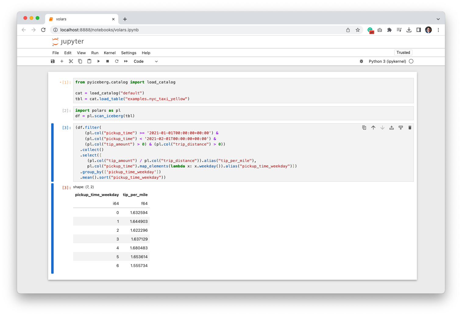
This is the well known NYC Taxi dataset. You can see that the table is partitioned by the pickup_time column, with applying the month transform. If you want to learn more on Icebergs’ hidden partitioning, please refer to the docs.
When we perform a query like:
df = pl.scan_iceberg(tbl)
df.filter(
    (pl.col("pickup_time") >= '2021-01-01T00:00:00+00:00') &
    (pl.col("pickup_time") < '2021-02-01T00:00:00+00:00')).collect()
The PyIceberg will evaluate the Arrow predicate, and prune away all the irrelevant months. Reducing the number of queries to S3, and speeding up the query. But most importantly, it keeps the table scalable and easy to query for non-distributed computing engines like Polars. It does not scan the whole table, or requires a special predicate for the partitioning, helping the user to access the data easily, without having to be an expert on the query engine, or how the data is laid out on the object store.

Hope this helps in your journey in adopting Iceberg. If you want to get involved, please check out the PyIceberg repository. We’re continuously working on improvements with respect to new features and performance, and feel free to reach out on Slack on the #python channel!


